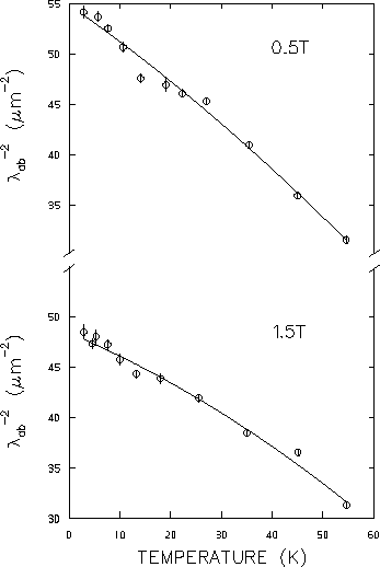
To determine the low temperature behaviour of
![]() several
assumptions were made in the fitting procedure to reduce the number of
independent variables. To start with, the Ginzburg-Landau parameter
several
assumptions were made in the fitting procedure to reduce the number of
independent variables. To start with, the Ginzburg-Landau parameter
![]() was assumed to be independent of temperature.
Although this is strictly valid only for weak coupling s-wave superconductors
away from Tc,
the lineshapes are not very sensitive to
was assumed to be independent of temperature.
Although this is strictly valid only for weak coupling s-wave superconductors
away from Tc,
the lineshapes are not very sensitive to ![]() in the
low-field region being considered here. Determining a value for
in the
low-field region being considered here. Determining a value for ![]() was accomplished by first fitting the recorded asymmetry spectra with
was accomplished by first fitting the recorded asymmetry spectra with
![]() as a fixed quantity. The value of
as a fixed quantity. The value of ![]() which minimized the
sum of the
which minimized the
sum of the ![]() 's for each temperature considered was then taken to
be the best value for
's for each temperature considered was then taken to
be the best value for ![]() .
The value
.
The value
![]() gave the best
overall fit to both the 0.5T and 1.5T data. Increasing
gave the best
overall fit to both the 0.5T and 1.5T data. Increasing ![]() to
73 was found to change
to
73 was found to change
![]() by less than 0.3nm.
The value
by less than 0.3nm.
The value
![]() is close to the value
is close to the value
![]() determined
from previous lineshape measurements on similar crystals in higher
magnetic fields [77].
determined
from previous lineshape measurements on similar crystals in higher
magnetic fields [77].
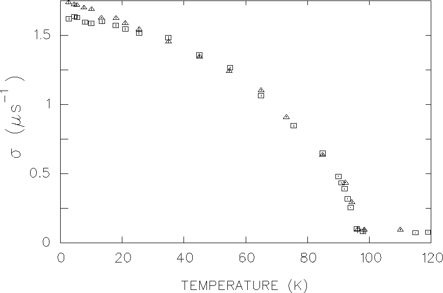
Fits to the early part of the signal ( i.e. the first ![]() s)
for data below Tc using an
equation in the form of Eq. (4.1) with a single gaussian
relaxation function of the form
s)
for data below Tc using an
equation in the form of Eq. (4.1) with a single gaussian
relaxation function of the form
![]() and
and
![]() pertaining to the average internal field, provides a simplified
visual display of the dependence of the lineshape width on temperature.
It is straightforward to use the polarization function in
Eq. (4.1) to relate the relaxation parameter
pertaining to the average internal field, provides a simplified
visual display of the dependence of the lineshape width on temperature.
It is straightforward to use the polarization function in
Eq. (4.1) to relate the relaxation parameter ![]() to the
second moment
to the
second moment
![]() .
The relationship is
[68]
.
The relationship is
[68]
 |
(4) |
 |
(5) |
 |
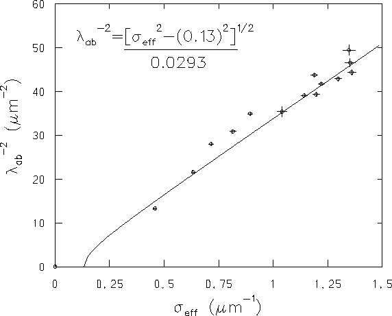
A more precise treatment of the data using the phenomenological model
of Eq. (3.39), holds the two parameters
![]() and
and
![]() accountable for the width of the measured field
distribution in the sample. Clearly these two parameters must combine
to mimic the behaviour in Fig. 4.6. Since
accountable for the width of the measured field
distribution in the sample. Clearly these two parameters must combine
to mimic the behaviour in Fig. 4.6. Since
![]() and
and
![]() both contribute to the linewidth and both are
expected to be temperature dependent quantities, the two parameters
cannot be treated as independent of one another when analyzing the
data. Indeed, fits to the data in which both parameters
were free to vary have
both contribute to the linewidth and both are
expected to be temperature dependent quantities, the two parameters
cannot be treated as independent of one another when analyzing the
data. Indeed, fits to the data in which both parameters
were free to vary have
![]() and
and
![]() playing off one another as
in Fig. 4.7. A temperature point which appears locally high in the
playing off one another as
in Fig. 4.7. A temperature point which appears locally high in the
![]() vs. T plot,
appears locally low in the
vs. T plot,
appears locally low in the
![]() vs. T plot and vice versa. A plot of
vs. T plot and vice versa. A plot of
![]() vs.
vs.
![]() suggests a linear correlation between the two parameters
as shown in Fig. 4.8.
The solid curve through the points in Fig. 4.8
has the following form:
suggests a linear correlation between the two parameters
as shown in Fig. 4.8.
The solid curve through the points in Fig. 4.8
has the following form:
 |
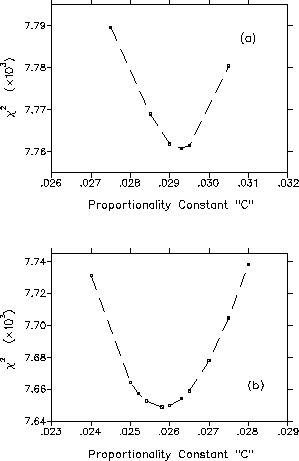 |
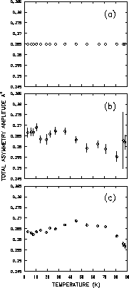
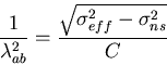
Figure 4.9 shows the total ![]() arising from global fits of the
0.5T and 1.5T data for various choices of the constant C.
The proportionality constant C was found to be
arising from global fits of the
0.5T and 1.5T data for various choices of the constant C.
The proportionality constant C was found to be
![]() and
and
![]() for
the 0.5T and 1.5T data, respectively.
The depolarization rate
for
the 0.5T and 1.5T data, respectively.
The depolarization rate
![]() was approximately
was approximately
![]() and
and
![]() for the 0.5T and 1.5T fields, respectively.
for the 0.5T and 1.5T fields, respectively.
In the first type of analysis, the total asymmetry amplitude ![]() for signals
recorded below Tc was fixed to the value of the precession amplitude
for signals
recorded below Tc was fixed to the value of the precession amplitude
![]() obtained from fitting data
above the transition temperature, prior to determining C
in Eq. (4.6).
Below Tc the asymmetry amplitude of the measured signal
obtained from fitting data
above the transition temperature, prior to determining C
in Eq. (4.6).
Below Tc the asymmetry amplitude of the measured signal ![]() is the sum of
the precession amplitude of the background signal
(
is the sum of
the precession amplitude of the background signal
(
![]() )
and
the precession amplitude of the signal originating from within the
sample (
)
and
the precession amplitude of the signal originating from within the
sample (
![]() ). Thus, here we are assuming that
the total precession amplitude of the resultant signal is
independent of temperature,
but dependent upon the applied magnetic field. The
asymmetry amplitude above Tcat fields of 0.5T and 1.5T were found to be
). Thus, here we are assuming that
the total precession amplitude of the resultant signal is
independent of temperature,
but dependent upon the applied magnetic field. The
asymmetry amplitude above Tcat fields of 0.5T and 1.5T were found to be
![]() and
and
![]() ,
respectively. The
field dependence is primarily attributed to the finite timing resolution of the
counters, which causes the observed precession amplitude to decrease
as the period of the muon precession becomes comparable to the timing
resolution.
,
respectively. The
field dependence is primarily attributed to the finite timing resolution of the
counters, which causes the observed precession amplitude to decrease
as the period of the muon precession becomes comparable to the timing
resolution.
In the final step of this
analysis, the status of the fitting parameters
was then as follows:
1. Sample Signal [refer to Eq. (3.39)]:
Variable parameters:
i) The amplitude
![]()
ii)
![]()
iii) The average internal field
![]()
iv) The initial phase ![]()
Fixed parameters:
i) ![]()
ii)
![]() fixed to
fixed to
![]() according to Eq. (4.6)
according to Eq. (4.6)
2. Background Signal [refer to Eq. (4.3)]:
Variable parameters:
i) The field
![]()
ii)
![]()
iii) The initial phase ![]() (same as for sample signal)
(same as for sample signal)
Fixed parameters:
i) The amplitude,
![]()
Thus in the final fit of the data there were six independent parameters.
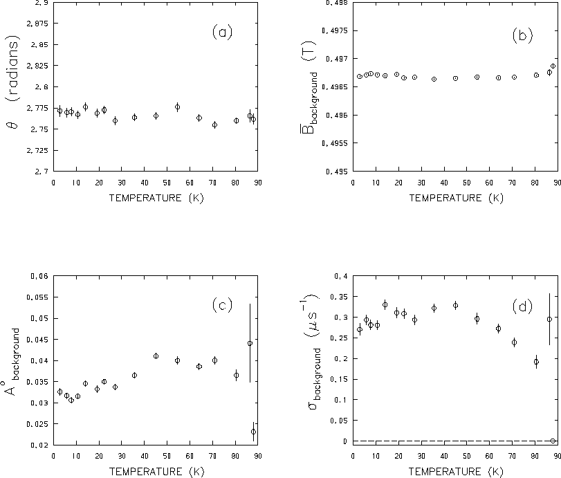
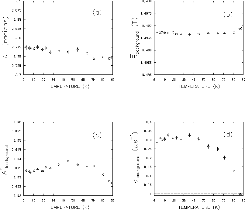
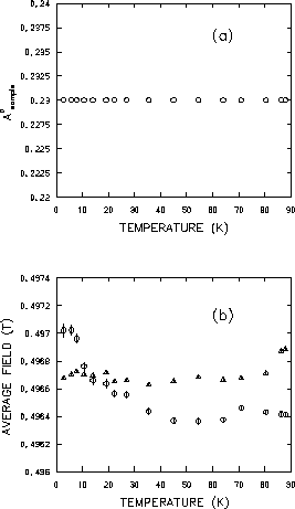
Figure 4.10 shows the variation with temperature
of the initial phase ![]() ,
the
average field
,
the
average field
![]() ,the amplitude
,the amplitude
![]() and
relaxation rate
and
relaxation rate
![]() of the background precession
signal, obtained from
fits of the 0.5T data. As indicated in Fig. 4.10(a),
the phase of the
initial muon spin polarization remains nearly constant throughout the
temperature scan ( i.e.
of the background precession
signal, obtained from
fits of the 0.5T data. As indicated in Fig. 4.10(a),
the phase of the
initial muon spin polarization remains nearly constant throughout the
temperature scan ( i.e.
![]() rad).
This implies that there were no appreciable fluctuations
in the applied field or electronics.
The nearly constant field
rad).
This implies that there were no appreciable fluctuations
in the applied field or electronics.
The nearly constant field
![]() in Fig. 4.10(b)
is a further indication of a highly stable applied
magnetic field.
The 1.5T data is not shown because there was a significant
change in the applied field after 40K.
in Fig. 4.10(b)
is a further indication of a highly stable applied
magnetic field.
The 1.5T data is not shown because there was a significant
change in the applied field after 40K.
Figure 4.10(d) shows a significant
drop in the relaxation rate of the
background signal at higher temperatures, indicating some temperature
dependence for
![]() .
However, at lower temperatures
(
.
However, at lower temperatures
(![]() K) the background relaxation rate
and hence the contribution of the background signal to
the second moment exhibits no obvious
correlation with temperature. This suggests that
K) the background relaxation rate
and hence the contribution of the background signal to
the second moment exhibits no obvious
correlation with temperature. This suggests that
![]() plays little role in the temperature dependence of
plays little role in the temperature dependence of ![]() in
Fig. 4.6. The fact that
in
Fig. 4.6. The fact that
![]() suggests
that the background is caused by a material with a large nuclear dipolar
interaction such as Cu, or is in a region of fairly large field inhomogeneity.
suggests
that the background is caused by a material with a large nuclear dipolar
interaction such as Cu, or is in a region of fairly large field inhomogeneity.
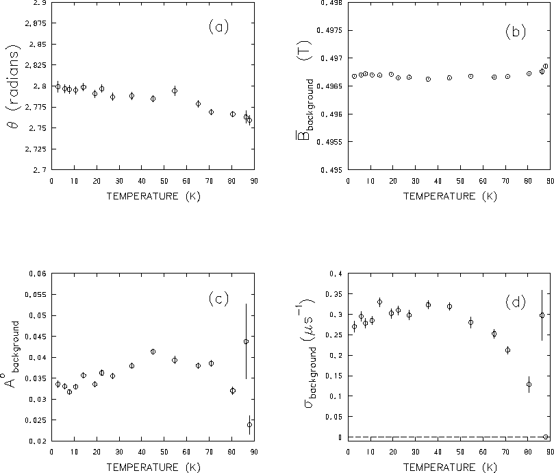 |
Figure 4.11 and Fig. 4.12
show the temperature dependence of
![]() ,
,
![]() and
and
![]() arising from
the same fits which produced the results in Fig. 4.10.
Together these parameters
constitute three of the four variable parameters (the other
being
arising from
the same fits which produced the results in Fig. 4.10.
Together these parameters
constitute three of the four variable parameters (the other
being ![]() )
which pertain to the signal originating from the sample.
The sample amplitude
)
which pertain to the signal originating from the sample.
The sample amplitude
![]() depicted in Fig. 4.11(a) shows
some scatter and a slight decrease at higher temperatures. The scatter
in the asymmetry amplitude is not all that surprising considering that the
data was recorded over a period of 5 days, through which time, small
fluctuations in experimental conditions were unavoidable. For instance,
one such experimental variation was the rate at which 4He was
pumped through the cryostat. At higher temperatures (where the required
cooling power is low) the amount of 4He flowing into the cryostat
and the corresponding pumping rate were minimized in an effort to
keep the heater voltage small to preserve the supply of
4He and to reduce thermal gradients between the thermometers
and the sample.
However, to maintain low temperatures a much larger flow of
4He was required. The increased density of helium atoms in the
cryostat increases the probability of scattering the incoming muons
before they can reach the sample, thus increasing the background signal
and decreasing the magnitude of
depicted in Fig. 4.11(a) shows
some scatter and a slight decrease at higher temperatures. The scatter
in the asymmetry amplitude is not all that surprising considering that the
data was recorded over a period of 5 days, through which time, small
fluctuations in experimental conditions were unavoidable. For instance,
one such experimental variation was the rate at which 4He was
pumped through the cryostat. At higher temperatures (where the required
cooling power is low) the amount of 4He flowing into the cryostat
and the corresponding pumping rate were minimized in an effort to
keep the heater voltage small to preserve the supply of
4He and to reduce thermal gradients between the thermometers
and the sample.
However, to maintain low temperatures a much larger flow of
4He was required. The increased density of helium atoms in the
cryostat increases the probability of scattering the incoming muons
before they can reach the sample, thus increasing the background signal
and decreasing the magnitude of
![]() .
To minimize this
effect, the cryostat sample space was pumped on hard, but the choice
of a specific combination of 4He-flow rate and the pumping rate was
purely judgemental. This is a possible explanation for the scatter
observed in Fig. 4.11(a). However, the downward trend of
.
To minimize this
effect, the cryostat sample space was pumped on hard, but the choice
of a specific combination of 4He-flow rate and the pumping rate was
purely judgemental. This is a possible explanation for the scatter
observed in Fig. 4.11(a). However, the downward trend of
![]() as one increases the temperature may be purely
statistical, as a similar behaviour was not observed
in more recently recorded data fitted with the same procedure.
Recall that since the total asymmetry amplitude was fixed, the variation
of
as one increases the temperature may be purely
statistical, as a similar behaviour was not observed
in more recently recorded data fitted with the same procedure.
Recall that since the total asymmetry amplitude was fixed, the variation
of
![]() with temperature in Fig. 4.10(c)
appears as a mirror image of Fig. 4.11(a).
with temperature in Fig. 4.10(c)
appears as a mirror image of Fig. 4.11(a).
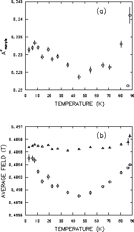 |
Figure 4.11(b) shows the temperature variation of the average
internal field
![]() experienced by muons implanted in the
experienced by muons implanted in the
![]() sample. For comparison,
the background field
sample. For comparison,
the background field
![]() is also plotted in Fig. 4.11(b).
In general, the field at any point in the sample is
the sum of the local fields in Eq. (3.13).
For all temperatures,
is also plotted in Fig. 4.11(b).
In general, the field at any point in the sample is
the sum of the local fields in Eq. (3.13).
For all temperatures,
![]() is less than
is less than
![]() ,
but
,
but
![]() appears to approach
appears to approach
![]() at both
ends of the temperature scan. In the high-temperature regime the vortex
cores begin to overlap with the internal field distribution approaching
full penetration of the applied field. Thus it is not surprising to see
the average internal field
at both
ends of the temperature scan. In the high-temperature regime the vortex
cores begin to overlap with the internal field distribution approaching
full penetration of the applied field. Thus it is not surprising to see
the average internal field
![]() approach
approach
![]() as one increases the temperature towards Tc.
The rise in average field
as one increases the temperature towards Tc.
The rise in average field
![]() at low temperatures, however, is
more difficult to understand.
Such an increase has also been reported in previous
work by Riseman [77]
and observed in more recent data taken at different
fields. The cause for such behaviour is puzzling indeed.
However, Fig. 4.11(b) is consistent with the time spectrum
shown in Fig. 4.3
which shows a more distinct beat in the muon spin precession signal at the
intermediate temperature T=35.5K, corresponding to a greater
separation between the average precession frequency of muons subjected
to the internal field distribution
and the average precession frequency of muons in the background field.
This suggests that the
increase in
at low temperatures, however, is
more difficult to understand.
Such an increase has also been reported in previous
work by Riseman [77]
and observed in more recent data taken at different
fields. The cause for such behaviour is puzzling indeed.
However, Fig. 4.11(b) is consistent with the time spectrum
shown in Fig. 4.3
which shows a more distinct beat in the muon spin precession signal at the
intermediate temperature T=35.5K, corresponding to a greater
separation between the average precession frequency of muons subjected
to the internal field distribution
and the average precession frequency of muons in the background field.
This suggests that the
increase in
![]() at low
temperatures may be due to some intrinsic phenomenon of the
at low
temperatures may be due to some intrinsic phenomenon of the
![]() sample itself.
sample itself.
Figure 4.12 shows the
temperature dependence of
![]() (which
in the phenomenological London Model is directly
proportional to the superfluid density ns) for the applied field
of 0.5T . Since the relaxation rate
(which
in the phenomenological London Model is directly
proportional to the superfluid density ns) for the applied field
of 0.5T . Since the relaxation rate
![]() is assumed
proportional to
is assumed
proportional to
![]() [see Eq. (4.6)], the
variation of
[see Eq. (4.6)], the
variation of
![]() with temperature resembles the behaviour
in Fig. 4.12.
Figure 4.13 shows the
low-temperature dependence of
with temperature resembles the behaviour
in Fig. 4.12.
Figure 4.13 shows the
low-temperature dependence of
![]() for both 0.5T and 1.5T applied fields.
As shown,
the presence of a linear term ( i.e.
for both 0.5T and 1.5T applied fields.
As shown,
the presence of a linear term ( i.e.
![]() )
in the low-temperature region is unmistakeable
for both 0.5T and 1.5T fields,
with the latter showing a weaker linear dependence
on T. A fit to the low-temperature data ( i.e. below 55K), with an
equation of the form:
)
in the low-temperature region is unmistakeable
for both 0.5T and 1.5T fields,
with the latter showing a weaker linear dependence
on T. A fit to the low-temperature data ( i.e. below 55K), with an
equation of the form:
 |
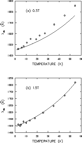
In Fig. 4.14 the temperature dependence of
![]() at
0.5T and 1.5T is shown. The solid curves represent microwave
measurements of the change in penetration depth
at
0.5T and 1.5T is shown. The solid curves represent microwave
measurements of the change in penetration depth
![]() taken in zero static magnetic field by Hardy et al. [6].
For the purpose of comparison,
taken in zero static magnetic field by Hardy et al. [6].
For the purpose of comparison,
![]() for each field is
chosen to be the value obtained from fitting the
for each field is
chosen to be the value obtained from fitting the ![]() SR
low-temperature data with Eq. (4.7). Surprisingly, the
microwave data shows a much better agreement with the
SR
low-temperature data with Eq. (4.7). Surprisingly, the
microwave data shows a much better agreement with the
![]() SR data at the higher magnetic
field of 1.5T.
SR data at the higher magnetic
field of 1.5T.
 |
There was some concern after completion of the above analysis that fixing
the total asymmetry amplitude to the value above Tcmay introduce systematic errors by
constraining the fits. The large fluctuation in the amplitude
of the muon spin precession signal originating
from the sample [see Fig. 4.11(a)]
was the source of such concerns. Intuitively, we expect that
![]() should
scale with the percentage of muons striking the sample. The fluctuations
in this percentage during the actual experiment were probably not large
enough to account for the large scatter in Fig. 4.11(a). If one
dismisses the previous explanation for the large fluctuations in
should
scale with the percentage of muons striking the sample. The fluctuations
in this percentage during the actual experiment were probably not large
enough to account for the large scatter in Fig. 4.11(a). If one
dismisses the previous explanation for the large fluctuations in
![]() ,
it is worth investigating this matter further.
,
it is worth investigating this matter further.
Since
![]() is not expected to change significantly over
the temperature scan, the data was refitted first by designating
is not expected to change significantly over
the temperature scan, the data was refitted first by designating
![]() and
and
![]() as variable parameters.
As in the previous analysis,
as variable parameters.
As in the previous analysis,
![]() was assumed to be proportional
to
was assumed to be proportional
to
![]() through Eq. (4.6). The proportionality
constant C was determined to be
0.0250(10) and
through Eq. (4.6). The proportionality
constant C was determined to be
0.0250(10) and
![]() for the 0.5T and 1.5T data
respectively. The variable parameters pertaining to the background
precession signal varied with temperature according to
Fig. 4.15. Comparing with Fig. 4.10, the phase
for the 0.5T and 1.5T data
respectively. The variable parameters pertaining to the background
precession signal varied with temperature according to
Fig. 4.15. Comparing with Fig. 4.10, the phase
![]() shifts down
shifts down
![]() rad, while
rad, while
![]() shifts upward
shifts upward
![]() mT. The degree of fluctuation in both these parameters
appears similar to that of the previous analysis, so again it seems
apparent that there were negligible fluctuations in the applied field.
mT. The degree of fluctuation in both these parameters
appears similar to that of the previous analysis, so again it seems
apparent that there were negligible fluctuations in the applied field.
 |
The amplitude
![]() and the
relaxation rate
and the
relaxation rate
![]() [see Fig. 4.15(c)
and Fig. 4.15(d)] show almost
no change from the results depicted in Fig. 4.10. Even the
size of the statistical error bars are comparable. These results indicate
that the fitting program is capable of clearly separating the unwanted
background signal from the sample signal.
[see Fig. 4.15(c)
and Fig. 4.15(d)] show almost
no change from the results depicted in Fig. 4.10. Even the
size of the statistical error bars are comparable. These results indicate
that the fitting program is capable of clearly separating the unwanted
background signal from the sample signal.
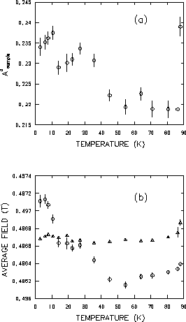
Figure 4.16(a) shows the temperature dependence of the amplitude
![]() corresponding to the muon spin precession signal
originating from the sample. The downward trend
with increasing T appears slightly more prominent
than in Fig. 4.11(a). The temperature dependence of
corresponding to the muon spin precession signal
originating from the sample. The downward trend
with increasing T appears slightly more prominent
than in Fig. 4.11(a). The temperature dependence of
![]() in Fig. 4.16(b) is significantly different from that in the previous
analysis. The average field
in Fig. 4.16(b) is significantly different from that in the previous
analysis. The average field
![]() is greater than
is greater than
![]() at the lowest of temperatures and does
not dip as far below
at the lowest of temperatures and does
not dip as far below
![]() as in Fig. 4.11(b) for temperatures
beyond this. At the high-temperature end in Fig. 4.11(b),
as in Fig. 4.11(b) for temperatures
beyond this. At the high-temperature end in Fig. 4.11(b),
![]() recovers to approximately the same value as in Fig. 4.11(b).
Again the rise in
recovers to approximately the same value as in Fig. 4.11(b).
Again the rise in
![]() at low
temperatures is surprising. It is possible that this is an effect due to
at low
temperatures is surprising. It is possible that this is an effect due to
![]() -
-![]() anisotropy. The presence of
anisotropy. The presence of ![]() -
-![]() anisotropy would distort the
vortex lattice into isoceles triangles as shown
in Fig. 3.9. If this lattice were to be modelled by one
consisting of equilateral triangles as assumed in our analysis, then
there would be some error in the determination of the average field
anisotropy would distort the
vortex lattice into isoceles triangles as shown
in Fig. 3.9. If this lattice were to be modelled by one
consisting of equilateral triangles as assumed in our analysis, then
there would be some error in the determination of the average field
![]() .
This would be a greater problem at low temperatures where the cores are
further apart and errors in spectral weighting are more pronounced.
.
This would be a greater problem at low temperatures where the cores are
further apart and errors in spectral weighting are more pronounced.
 |
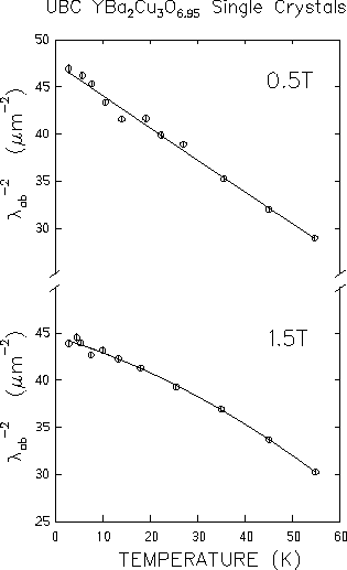
The low-temperature dependence of
![]() is shown in
Fig. 4.17. Surprisingly, the scatter in the data points
is not significantly greater than in Fig. 4.13. Noticeably
different however, is an increase in the linear term (see Table 4.1).
Furthermore, fits to Eq. (4.6) yield
is shown in
Fig. 4.17. Surprisingly, the scatter in the data points
is not significantly greater than in Fig. 4.13. Noticeably
different however, is an increase in the linear term (see Table 4.1).
Furthermore, fits to Eq. (4.6) yield
![]() Å and
Å and
![]() Å for the 0.5T and 1.5T data,
respectively. A comparison to the microwave measurements of Hardy et al.,
assuming these values for
Å for the 0.5T and 1.5T data,
respectively. A comparison to the microwave measurements of Hardy et al.,
assuming these values for
![]() is shown in Fig. 4.18.
There appears to be even less agreement at 0.5T than previously noted in
Fig. 4.14(a). However, the agreement at
1.5T in Fig. 4.18(b)
is comparable to that in Fig. 4.14(b) despite the significant
difference in
is shown in Fig. 4.18.
There appears to be even less agreement at 0.5T than previously noted in
Fig. 4.14(a). However, the agreement at
1.5T in Fig. 4.18(b)
is comparable to that in Fig. 4.14(b) despite the significant
difference in
![]() .
.
 |
 |
As a final step in the analysis, the data was refitted with the amplitude
![]() fixed to the average value of the data below 55K
in Fig. 4.16(a). This results in a noticeable reduction
in the scatter for the parameters
fixed to the average value of the data below 55K
in Fig. 4.16(a). This results in a noticeable reduction
in the scatter for the parameters
![]() and
and
![]() (see Fig. 4.19). Fixing
(see Fig. 4.19). Fixing
![]() in this way significantly shifts the data points
above 40K. This is not surprising since
in this way significantly shifts the data points
above 40K. This is not surprising since
![]() was
fixed to the low-temperature average. The phase
was
fixed to the low-temperature average. The phase ![]() shows a
slight decrease at high temperatures [see Fig. 4.19(a)] and
shows a
slight decrease at high temperatures [see Fig. 4.19(a)] and
![]() levels off above 40K [see Fig. 4.20(b)]. These results
suggest that fixing
levels off above 40K [see Fig. 4.20(b)]. These results
suggest that fixing
![]() to the low-temperature average
reduces the scatter in the low-temperature data, but
it is not yet clear whether or not we are introducing non-physical
deviations in the high-temperature region.
to the low-temperature average
reduces the scatter in the low-temperature data, but
it is not yet clear whether or not we are introducing non-physical
deviations in the high-temperature region.
 |
 |
The reduction in scatter is most noticeable in Fig. 4.21 which
shows the temperature dependence of
![]() .
From
Eq. (4.6) we find
.
From
Eq. (4.6) we find
![]() Å and
Å and
![]() Å for the 0.5T and 1.5T data,
respectively. A plot of the temperature dependence of
Å for the 0.5T and 1.5T data,
respectively. A plot of the temperature dependence of
![]() over the full temperature scan is shown in Fig. 4.22. The
two fields appear to converge well before Tc, but the crossover is
difficult to determine.
As shown in Fig. 4.23, there is improved
agreement between the microwave measurements
and the 0.5T
over the full temperature scan is shown in Fig. 4.22. The
two fields appear to converge well before Tc, but the crossover is
difficult to determine.
As shown in Fig. 4.23, there is improved
agreement between the microwave measurements
and the 0.5T ![]() SR data, while the agreement with the
1.5T data is comparable to that of the previous two fitting methods.
The total asymmetry amplitude of the muon spin precession signal as determined
from all three fitting procedures is shown in Fig. 4.24. It
appears as though one is justified in fixing the total asymmetry amplitude,
as the average values are comparable.
SR data, while the agreement with the
1.5T data is comparable to that of the previous two fitting methods.
The total asymmetry amplitude of the muon spin precession signal as determined
from all three fitting procedures is shown in Fig. 4.24. It
appears as though one is justified in fixing the total asymmetry amplitude,
as the average values are comparable.
 |
 |
 |
The results from all three types of analysis are summarized in Table 4.1. Methods (ii) and (iii) give comparable results, but differ substantially from method (i). The difference appears to be related to the proportionality constant C of Eq. (
![\begin{displaymath}\frac{1}{\lambda_{ab}^{2}(T)} = \frac{1}{\lambda_{ab}^{2}(0)} \left[
1 - \alpha T - \beta T^{2} \right]
\end{displaymath}](img390.gif)