


Next: 2.5 Measuring the Characteristic
Up: 2 The Characteristic Length
Previous: 2.3.3 Nonlinear and Nonlocal
The temperature and magnetic field dependence of both the penetration
depth and coherence length appear quite naturally
in Ginzburg-Landau (GL) theory [41].
Like the London model, the GL model is independent of
the underlying mechanism for superconductivity.
However, it must be emphasized that
GL theory is strictly valid only near the normal-to-superconducting
phase boundary, and is thus not generally applicable at low temperatures.
In the theory,
a complex order parameter  is introduced,
where is a function of temperature, magnetic field and the spatial
coordinates. Ginzburg and Landau assumed that near Tc where
is small, the free-energy difference per unit volume
between the normal and
superconducting state at zero magnetic field
may be expanded as a function of
is introduced,
where is a function of temperature, magnetic field and the spatial
coordinates. Ginzburg and Landau assumed that near Tc where
is small, the free-energy difference per unit volume
between the normal and
superconducting state at zero magnetic field
may be expanded as a function of
| 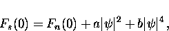 |
(50) |
where a and b are temperature-dependent coefficients such that near
Tc
where a0 and b0 are positive coefficients, so that
 below Tc.
Minimizing the free energy with respect to
below Tc.
Minimizing the free energy with respect to  gives
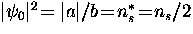
the zero-field value of the order parameter
gives
the zero-field value of the order parameter
| 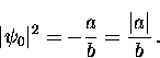 |
(51) |
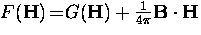
In the presence of a magnetic field, the free energy in the superconducting
state is increased. In particular, the work
done on the sample by the magnetic field  is
is
| 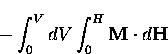 |
(52) |
where V is the volume of the sample and  is the sample
magnetization. In the Meissner phase,
is the sample
magnetization. In the Meissner phase,  so that
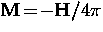 , whereas in the normal state
is essentially zero.
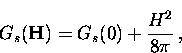
This means that the Gibbs free energy per unit volume
in the superconducting state
increases in the presence of a magnetic field to
, whereas in the normal state
is essentially zero.
This means that the Gibbs free energy per unit volume
in the superconducting state
increases in the presence of a magnetic field to
|  |
(53) |
whereas in the normal state
| 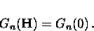 |
(54) |
At the phase change, 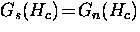 where Hc is the critical
field. Thus, using Eq. (2.56) and Eq. (2.57), one has
where Hc is the critical
field. Thus, using Eq. (2.56) and Eq. (2.57), one has
|  |
(55) |
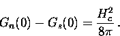
Using the Legendre transformation
 ,Eq. (2.58) may be written in terms of the Helmholtz free
energy per unit volume
,Eq. (2.58) may be written in terms of the Helmholtz free
energy per unit volume
| 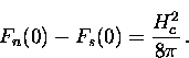 |
(56) |
This implies that an energy  , called the ``condensation
energy'', is given up by the formation of the superconducting
state.
, called the ``condensation
energy'', is given up by the formation of the superconducting
state.
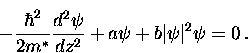
Assuming that the order parameter is not completely rigid
in the presence of a magnetic field, there is
an additional energy term associated with variations in .This term was assumed by Ginzburg and Landau to take the form
| 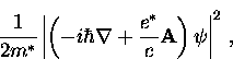 |
(57) |
where later it was found that  and
and  .Thus, the total free energy per unit volume of the superconducting
state in the presence of a magnetic field is
.Thus, the total free energy per unit volume of the superconducting
state in the presence of a magnetic field is
Minimizing this expression with respect to
leads to the ``first GL equation''
| 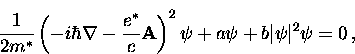 |
(58) |
and with respect to  , the ``second GL equation''
| 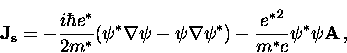 |
(59) |
which is the standard expression for the quantum-mechanical
current. This equation has the same form as the London
equation, except that is spatially varying.
The GL equations can be solved analytically for
simple cases only.
Consider a superconductor in a weak magnetic field with the sample
dimensions much greater than the magnetic penetration depth.
To first order in B,
in Eq. (2.63) can be replaced by its equilibrium
zero-field value  from Eq. (2.54)
| 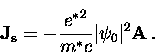 |
(60) |
Taking the curl of both sides of this equation gives
| 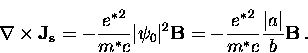 |
(61) |
Using Eq. (2.12), this can be rewritten as
|  |
(62) |
which, upon comparing to the expression in Eq. (2.13), gives
|  |
(63) |
which is the same as the London penetration depth if
 .
.
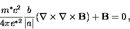
Consider a second example where varies only in the
 -direction, but the applied
magnetic field is zero.
In this case the first GL equation becomes
-direction, but the applied
magnetic field is zero.
In this case the first GL equation becomes
|  |
(64) |
Assuming is real, we can introduce a dimensionless
order parameter
| 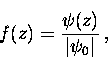 |
(65) |
where  is given by Eq. (2.54). Thus,
Eq. (2.68) becomes
is given by Eq. (2.54). Thus,
Eq. (2.68) becomes
| 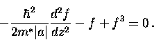 |
(66) |
A natural length scale for spatial varitaions of the order
parameter is thus
| 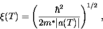 |
(67) |
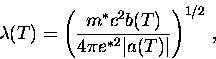
which is known as the GL coherence length.
Note that both the GL coherence length and the GL penetration depth
are temperature dependent quantities.
From Eq. (2.53) it is clear that both  and
and
 vary as (1-T/Tc)-1/2 with temperature, so that
their ratio is independent of temperature
vary as (1-T/Tc)-1/2 with temperature, so that
their ratio is independent of temperature
| 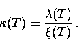 |
(68) |
 is known as the ``GL parameter''.
A precise calculation from the microscopic theory
gives a weak temperature dependence for , with increasing
as T decreases [42].
In GL theory, a superconductor is called ``type-I''
if
is known as the ``GL parameter''.
A precise calculation from the microscopic theory
gives a weak temperature dependence for , with increasing
as T decreases [42].
In GL theory, a superconductor is called ``type-I''
if  and ``type-II'' if
  .When the order parameter throughout the sample is essentially a constant,
the GL model reduces to the London model. This occurs
when
.When the order parameter throughout the sample is essentially a constant,
the GL model reduces to the London model. This occurs
when  , which is the case for the
high-Tc superconductors.
, which is the case for the
high-Tc superconductors.
GL theory is particularly useful in modelling the small variation of  with magnetic field found near Tc.
Pippard [31] first used a simple thermodynamic argument,
which distributes the entropy difference due
to changes in H over a layer of thickness
with magnetic field found near Tc.
Pippard [31] first used a simple thermodynamic argument,
which distributes the entropy difference due
to changes in H over a layer of thickness  , to
explain the field dependence of he observed in the type-I
superconductor Sn.
Historically, this marks the introduction of as a fundamental length scale in superconductivity theory.
Although the field dependence is built into the GL theory,
for arbitrary H, has a non-negligible dependence on field.
Thus, in general, the field dependence of both and
must be obtained by numerically
solving the complete nonlinear GL equations.
Analytical results can be obtained in special cases, such as for thin films.
, to
explain the field dependence of he observed in the type-I
superconductor Sn.
Historically, this marks the introduction of as a fundamental length scale in superconductivity theory.
Although the field dependence is built into the GL theory,
for arbitrary H, has a non-negligible dependence on field.
Thus, in general, the field dependence of both and
must be obtained by numerically
solving the complete nonlinear GL equations.
Analytical results can be obtained in special cases, such as for thin films.
Next: 2.5 Measuring the Characteristic
Up: 2 The Characteristic Length
Previous: 2.3.3 Nonlinear and Nonlocal