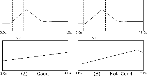
Figure 2.4: Example (A) shows how to rescale the graph to include just the segment of the data needed to get a best-fit line. In Example (B), too much of the data is included, and the best-fit line will not correspond to the desired segment of data.
Another method consists in using the software to calculate velocity based on a kind of average of a segment of the data, called a best fit line. To do this, you will first need to instruct the software which segment of data it should fit a line to. The software will fit a line to the entire segment of data shown on the graph, so to fit a line to just one part, you must rescale the graphs. Find the menu with the (R)escale option and hit `R' (you will have to exit the Cursor function, if you have not already done so, by pressing Return). A small cursor will appear in the upper-left corner of the upper graph. If you hit the space bar, it will move to the lower-right corner of the graph, and if you keep hitting the space bar it will move to these two corners of the second graph and then back to the top graph again. At each of these corners, you can use the arrow keys to adjust the scale of the graph: the up- and down-arrow keys will magnify or demagnify the vertical scale and the left- and right-arrow keys will magnify or demagnify the time scale. (Again, holding down the Control key will move things faster.) Note that the time scale will change on both graphs simultaneously, while the vertical scale changes separately for each graph. For now, you only need to be concerned with the horizontal rescaling -- that is, with changing the first and last time values on the graph so that you are looking at just a part of the data. By playing around with rescaling in the left and right corners of the graph, using just the left- and right-arrow keys, you can eventually arrange it so that the graphs show only that segment of time during which the rider is in constant motion toward the elastic bumper. It is not necessary here to try to include every single data-point from the beginning until the point of collision; rather, you should try to focus on some window of points reasonably inside this range, so that extraneous effects at the ends of this motion will not show up in the graph (see Fig. 2.4).

Figure 2.4:
Example (A) shows how to rescale the graph
to include just the segment of the data needed to
get a best-fit line. In Example (B),
too much of the data is included, and the
best-fit line will not correspond to
the desired segment of data.
When this is done, exit the Rescaling function by pressing Return. Find the menu with (B)est Fit Line and press `B'. The software draws a best fit line through the data points on each graph. It is something like the graphical equivalent of what happens when you take the average of several measurements. Using the information derived from a best-fit line should be more accurate than using individual data points, in the same way that using the average of several measurements of a quantity is more reliably accurate than using any single measurement.
At the bottom of the screen, the slopes of each of the best-fit lines are indicated by ``M = ....'' The slope of the displacement graph indicates a velocity, in this case the velocity of the rider moving toward the elastic bumper. The slope on the velocity graph indicates the acceleration. Are these what you expected them to be? How close is the velocity to what you measured for the velocity above?
Make a note of the velocity indicated by the best fit of the displacement graph and then rescale your windows so that only the smooth motion away from the elastic bumper and toward the Sonic Ranger is visible. Using the best-fit method again, find the velocity during this interval, and calculate the coefficient of restitution again. How would you explain any differences between the result of this calculation and the result of the method you used earlier? Which method do you think gives a more accurate value for e?
Using one of these methods, conduct several more trials and find an average value for e.